 All papers examples
Disciplines

- MLA
- APA
- Master's
- Undergraduate
- High School
- PhD
- Harvard
- Biology
- Art
- Drama
- Movies
- Theatre
- Painting
- Music
- Architecture
- Dance
- Design
- History
- American History
- Asian History
- Literature
- Antique Literature
- American Literature
- Asian Literature
- Classic English Literature
- World Literature
- Creative Writing
- English
- Linguistics
- Law
- Criminal Justice
- Legal Issues
- Ethics
- Philosophy
- Religion
- Theology
- Anthropology
- Archaeology
- Economics
- Tourism
- Political Science
- World Affairs
- Psychology
- Sociology
- African-American Studies
- East European Studies
- Latin-American Studies
- Native-American Studies
- West European Studies
- Family and Consumer Science
- Social Issues
- Women and Gender Studies
- Social Work
- Natural Sciences
- Anatomy
- Zoology
- Ecology
- Chemistry
- Pharmacology
- Earth science
- Geography
- Geology
- Astronomy
- Physics
- Agriculture
- Agricultural Studies
- Computer Science
- Internet
- IT Management
- Web Design
- Mathematics
- Business
- Accounting
- Finance
- Investments
- Logistics
- Trade
- Management
- Marketing
- Engineering and Technology
- Engineering
- Technology
- Aeronautics
- Aviation
- Medicine and Health
- Alternative Medicine
- Healthcare
- Nursing
- Nutrition
- Communications and Media
- Advertising
- Communication Strategies
- Journalism
- Public Relations
- Education
- Educational Theories
- Pedagogy
- Teacher's Career
- Statistics
- Chicago/Turabian
- Nature
- Company Analysis
- Sport
- Paintings
- E-commerce
- Holocaust
- Education Theories
- Fashion
- Shakespeare
- Canadian Studies
- Science
- Food Safety
- Relation of Global Warming and Extreme Weather Condition
Paper Types

- Movie Review
- Essay
- Admission Essay
- Annotated Bibliography
- Application Essay
- Article Critique
- Article Review
- Article Writing
- Assessment
- Book Review
- Business Plan
- Business Proposal
- Capstone Project
- Case Study
- Coursework
- Cover Letter
- Creative Essay
- Dissertation
- Dissertation - Abstract
- Dissertation - Conclusion
- Dissertation - Discussion
- Dissertation - Hypothesis
- Dissertation - Introduction
- Dissertation - Literature
- Dissertation - Methodology
- Dissertation - Results
- GCSE Coursework
- Grant Proposal
- Admission Essay
- Annotated Bibliography
- Application Essay
- Article
- Article Critique
- Article Review
- Article Writing
- Assessment
- Book Review
- Business Plan
- Business Proposal
- Capstone Project
- Case Study
- Coursework
- Cover Letter
- Creative Essay
- Dissertation
- Dissertation - Abstract
- Dissertation - Conclusion
- Dissertation - Discussion
- Dissertation - Hypothesis
- Dissertation - Introduction
- Dissertation - Literature
- Dissertation - Methodology
- Dissertation - Results
- Essay
- GCSE Coursework
- Grant Proposal
- Interview
- Lab Report
- Literature Review
- Marketing Plan
- Math Problem
- Movie Analysis
- Movie Review
- Multiple Choice Quiz
- Online Quiz
- Outline
- Personal Statement
- Poem
- Power Point Presentation
- Power Point Presentation With Speaker Notes
- Questionnaire
- Quiz
- Reaction Paper
- Research Paper
- Research Proposal
- Resume
- Speech
- Statistics problem
- SWOT analysis
- Term Paper
- Thesis Paper
- Accounting
- Advertising
- Aeronautics
- African-American Studies
- Agricultural Studies
- Agriculture
- Alternative Medicine
- American History
- American Literature
- Anatomy
- Anthropology
- Antique Literature
- APA
- Archaeology
- Architecture
- Art
- Asian History
- Asian Literature
- Astronomy
- Aviation
- Biology
- Business
- Canadian Studies
- Chemistry
- Chicago/Turabian
- Classic English Literature
- Communication Strategies
- Communications and Media
- Company Analysis
- Computer Science
- Creative Writing
- Criminal Justice
- Dance
- Design
- Drama
- E-commerce
- Earth science
- East European Studies
- Ecology
- Economics
- Education
- Education Theories
- Educational Theories
- Engineering
- Engineering and Technology
- English
- Ethics
- Family and Consumer Science
- Fashion
- Finance
- Food Safety
- Geography
- Geology
- Harvard
- Healthcare
- High School
- History
- Holocaust
- Internet
- Investments
- IT Management
- Journalism
- Latin-American Studies
- Law
- Legal Issues
- Linguistics
- Literature
- Logistics
- Management
- Marketing
- Master's
- Mathematics
- Medicine and Health
- MLA
- Movies
- Music
- Native-American Studies
- Natural Sciences
- Nature
- Nursing
- Nutrition
- Painting
- Paintings
- Pedagogy
- Pharmacology
- PhD
- Philosophy
- Physics
- Political Science
- Psychology
- Public Relations
- Relation of Global Warming and Extreme Weather Condition
- Religion
- Science
- Shakespeare
- Social Issues
- Social Work
- Sociology
- Sport
- Statistics
- Teacher's Career
- Technology
- Theatre
- Theology
- Tourism
- Trade
- Undergraduate
- Web Design
- West European Studies
- Women and Gender Studies
- World Affairs
- World Literature
- Zoology
Macroeconomics Questions, Statistics Problem Example
Hire a Writer for Custom Statistics problem
Use 10% Off Discount: "custom10" in 1 Click 👇
You are free to use it as an inspiration or a source for your own work.

Consumption and savings
We see an open economy in two seasons. The outputs Y1 and Y2 are delivered from the outside in each cycle. Increase the lifetime use of representative consumers
U = u(C1) + ?u(C2)
The consumption and ? in cycles C1 and C2 are subjective discount factors, 0 << 1. The country can borrow on the world market at a certain real interest rate. The initial attribute is zero. So let’s write the budget ban

Solve for consumption in the current period
Use solution alternative methods (use Logrange method if needed). Solving C2’s budget barriers
| C2 = Y1(1 + r) + Y2 ? (1 + r)C1
substitute given constraint into give objective function |
(1) |
| U = u(C1) + ?u(Y1(1 + r) + Y2 ? (1 + r)C1)
Maximize given objective function C1. |
(2) |
The FOC is

The left side of the last exposure is the ratio of the exchange rate (MRS) between the first and the second stage consumption, that is, how much C1 you are willing to convert to a unit of C2 (subject to standard usage). On the right is the comparative consumer price of the second stage, that is, how much C1 you have to give up to get C2 units. Best MRS (C1,C2)=relative price. If you can increase utility by trading C1 for C2 and vice versa if
Consumption Response
After converting the data from 1 to 3, we get an equation to determine the optimal period 1 consumption as a function of the external () variable. The optimal period is derived from two consumption equivalents.
1:). Substituting this into the objective function gives the indirect utility function, i.e. maximal utility as a function of exogenous variables
To see how welfare is affected by an increase in the interest rate we derive
In optimum the FOC holds, ) = 0, and we are left with
Empirical evidence
We find that the identity of the welfare effect (), i.e. the country depends on the identity of the borrower or the first () lender. If the country is a lender in the first period, rising interest rates will increase welfare. Note that an increase in interest rates is equivalent to a decrease in consumer prices during the second phase. If the country is a lender, the first stage is its consumption exports and the second stage is the consumption imports. Therefore, it is possible to improve the country’s trade terms (import prices) / (export prices) by lowering interest rates. Now, it pays more for exports and less for imports, and things are better in this country.
Understand the impact of trauma
The SoloW model can also be described as the previous (RPC) Real Business Cycle model. This model can be used to predict the economic response to productivity or taste shocks or government policy shocks.
Productivity (or taste) shock

The output is given by Yt = AtF (Kt, Lt) as the extreme form yt = Atf (kt), where At represents the total material production.
Remember the permanent negative impact on production work. G (k) and ? (k) function. The new default is empty. The economy is slowly changing from old to new.
If the effect level is moderate, changes in G (K) and ? (K) are also short-lived. Previously, capital and exports would fall to a lesser extent. However, production returns to the original level, capital and output begin to increase to the old height and fixed rates.
The effect of electric shock on t kt and yt is shown in Figure inside. The set line corresponds to the central center, and the line corresponds to the permanent shock.
Taste Shock: Consider a temporary decrease in storage rate. (K). What happens when autumn is permanent?What is central mobility? The function drops slightly and returns to its original state
The model and the data
How does the RPC model fit the fashion model?
According to the business cycle and competition cycle testing methods, there are some specific principles.
Answer: Money is not very important in the business cycle.
The business cycle is generated by the optimal response of rational agents to actual vibrations, and actual vibrations are usually fluctuations in output growth. But prices or government procurement priorities will fluctuate around.
It is often useful to create a model using simulation. Usually this takes the form of generating a series of random observations. (Usually based on a specific statistical distribution) The resulting observations can then be read using the remaining techniques described on this website. Monte Carlo simulations is the name to this
Excel functions: Excel provides two functions for generating random numbers.
RAND()-Generate a random number between 0 and 1.
RANDBETWEEN (a, b)-Generate a random integer between a and b.
[50, 150] The distance interval theorem is modeled by generating 50 samples and 100 dimensions uniformly distributed throughout the space. Therefore, each data element with a potential of 50 to 150 is selected in each model.
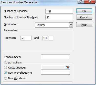
“Data”> “Analysis” | “Select Data Analyzer”, then select “Random Number Generation Data Analysis Tool”, in Figure 1.

Figure 1 dialog box FOR Random number generating
To delete an Excel project with 100 columns and 50 rows, we use the AVERAGE function to calculate the average value of each column. The result is an entry of 100 entries, which contains descriptions of each of the 100 types. As shown in Figure 2 (10×10 lines are adjusted to fit the screen).

Figure 2-100 random samples in materials
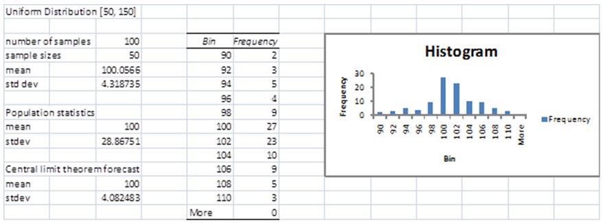
We now use the Excel histogram data analysis tool to create a chart containing 100 examples algorithms, as illustrated by right side of Figure 3.

Figure 3-Test of middle range hypothesis
The average deviation like algorithm is 100.0566, and the standard deviation is 4.318735. You can see that the bar graph is right by the bell curve of the normal distribution.
Since the sample is drawn from a uniform supply in the range of [50, 150], it can be observed from the uniform supply that the whole average = 100 and the stagnant is deviation = 28.86751.
Based on the middle range hypothesis, we wish that the average population of the illustration algorithm is average, which seems very close to 100.0566 100. We expect the model will also have standard deviation It is approximately the value of 4.318735.
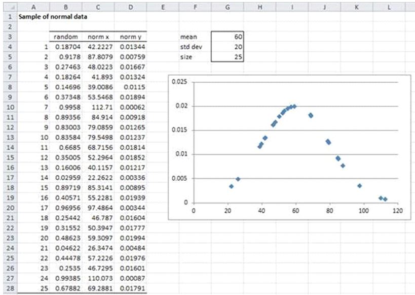
Note: You can manually create a random model that follows any distribution supported by Excel without using data analysis tools. E.g. To create a model of size 25 that follows a normal supply chain with a mean amount of 60 and a constant deviation of 20, just use the formula = NORMINV(RAND(), 60, 20).
We have done this in column C (the value column) of Figure 4. E.g. Cell C 4 contains the formula
= NORMINV (B4, $G$3, $G$4)
In column D, we find the probability (ie value), for example, the formula D4
= NORMDIST(C4, $G$3, $G$4, FALSE)
Finally, we create a scatter plot of x and y values ??that looks like a normally distributed hourly curve.
 Harvard
Figure 4-Create a model from a normal distribution
Observation: In a similar way, you can create random models for any distribution supported by Excel (or the actual statistical resource pack). E.g. To create an element with mean = 7 from the Poison distribution, we use the formula = POISSON_INV(RAND(), 7), where POISSON_INV is the actual statistical function described in the Poison distribution.
Random number weight
When using the Excel random number formula = RANDBETWEEN (1, 4), the probability of any value 1, 2, 3, or 4 is the same 25%. We now describe a way to change the likelihood of any particular value occurring.
Actual statistics function: The actual statistics resource package provides the following functions.
WRAND(R1) = a random integer between 1 and n, where R1 is the weight of the n×1 column.
Example 2: Using the weights in the range of H4: H7 in Figure 1, create 20 random numbers from {1, 2, 3, 4 sets.
Therefore, the probability of producing 1 is 50 / (50 + 10 + 20 + 20) = 50%, the probability of producing 2 is 10 / (50 + 10 + 20 + 20) = 10%, and so on.
The results are shown in column J of Figure 5.
Figure 5: The formation of weighted random numbers
For each cell in the range of J4:J23 has the formula =WRAND($H$4:$H$7). The number ??1, 2, 3, and 4 in the range L3: M7, J4: J23 indicate how many times each occurrence. As we have seen, the frequency is similar (but not the same) as the probability generated by the weight.
| strongly | weakly | Not at all | |||
| 1 | Investment is much more volatile than GDP. | / | |||
| 3 | .Employment (here hours worked) is less volatile than GDP | / | |||
| 4a. | Private consumption is strongly positively correlated GDP | / | / | ||
| 4b. | Investment in strongly positively correlated with GDP | / | |||
| 5a. | 5. Employment (here hours worked) is procyclical and | / | |||
| 5b. | 5 b. More strongly correlated with GDP than real wages and output per hour worked | / | |||
| 5c. | 5c. Output per hour is procyclical | ||||
| 5d. | 5d. Real wages are weakly correlated with GDP | / | / | ||
| 7. | 6. Employment (here hours worked) is a lagging variable | / | |||
| 8. | 7. GDP is persistent and consumption persistence is about the same | / | |||
| 9. | 8. Employment tends to be more persistent than GDP | / | |||
| 10a. | 9. Labour input varies in a strong procyclical manner, explaining most of the output gap | / | |||
| 10b. | 10. TFP also varies preocyclically | / | |||
How table does this version of the RBC model appear to illustrate the economy and how might it be improved?
This suggests that the representative agent design is not very important in solving policy problems in its essence. The biggest challenge of RBC theory is to create a more isolated model. Models with different intelligence have been developed (Jose-Victor Rios-Ral, 1994, research provided), but the differences introduced are very small — for example, in some formulas, the probability of working of employees is different, or some older, skilled workers, other young, incompetent: the actual business cycle is 1,779 employees. The scope of this model poses the most powerful technical problems, but it is necessary to make the research project more practical. 27 It is difficult to predict the final outcome of a research project. However, the final consensus is that although the RBC model cannot be accounted for by many changes in the timeline of the economy, the RBC theory will change the path of macroeconomics. The RBC theory has not significantly changed our view of the business cycle, but the development of this research project has also provided a fundamental change in the way we position the economy. It is embedded in a general equity model, which can calculate an economy that can display certain characteristics of real data sets. As the technological frontier progresses, these models can incorporate more and more realities. Such an example can be used with confidence to resolve all hope. Thus, the long-term contribution of real business cycle theory can prove to be a revolution in economic research and policy evaluation methods.

Stuck with your Statistics problem?
Get in touch with one of our experts for instant help!

Time is precious
don’t waste it!
writing help!


Plagiarism-free
guarantee

Privacy
guarantee

Secure
checkout

Money back
guarantee

