Statistical Signature Assignment, Essay Example

Relationship between Education and Gender 

The first question explores the relationship between education and gender.  In the substantial social science research corpus published on variables related to education and gender, results show a gap in education between men and women.  That is, men on average, have an overall higher level of education than women- although results vary by country and time frame examined (Mammen & Paxson, 2000).  In addition, this relationship is rapidly evolving, particularly in industrialized countries, as women enter institutions of higher education in increasing numbers (Mammen & Paxson, 2000).

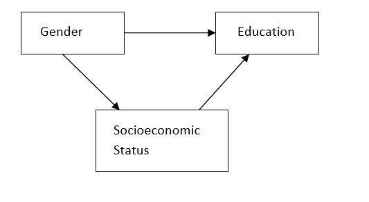
Having noted the general relationship, however, there are numerous caveats to it. For example, Jacobs (1996) performs a study examining the relationship between gender and access to higher education.  Jacobs introduces the main literature on the subject in which the relationship between gender and education is often times mediated by the social inequality (diagram 1). This potential relationship is important to note because in statistics often times there are numerous variables either mediating or confounding the relationship between two variables- this means one might not be measuring the putative relationship between two variables using statistical analysis.
Diagram 1: Relationship between Gender and Education mediated by Socioeconomic Status

In addition, Jacobs posits the relationship between education and gender is more complicated than often conceptualized. For example, while many studies traditionally show that men have an advantage in access and achievement, such findings are often too broad in nature, not undertaking proper stratification (Jacobs, 1996).  Jacobs finds that while men traditionally may have greater access to education (enrollment opportunities); women’s achievement in college exceeds men in numerous aspects meaning they may be better “educated.” Thus, when speaking about the relationship between gender and education, one must be careful how education is measured (access versus achievement) and potential mediators and confounders in the relationship.

In the provided data sample, gender is a categorical variable bifurcated into two different responses: 1) Male; 2) Female.  Education is operationalized as the highest year of school completed. After conducting basic descriptive statistics, the sample is predominantly female (56%, SD=2.83) with the number of males in the minority (44%, SD=2.94) (all output for this and other questions is placed in the paper’s appendix).  The data set is quite complete when examining gender and education- there are only 4 missing observations in gender and highest year of school completed.

Table 1: Gender and Education Sample Statistics

After conducting basic descriptive statistics, there is an existing concern over the nature of the dependent variable in this analysis: education. The variable “education in years” may not properly be considered a continuous variable or normally distributed. Indeed, regarding the concern over the variable’s continuous nature, education in years is not continuous because an individual cannot attend 12.25 or 15.5 years of school. One of the main assumptions for using a t-test is a continuous dependent variable- highest year of school completed in this data set is best described as an interval variable. That concern will temporarily be put aside in order to establish whether the dependent variable is normally distributed.  After conducting a number of tests including checking the kurtosis and skewness of the variable, it is roughly normally distributed.  The data for “highest year of school completed” is between the acceptable range of +2 and -2 for both kurtosis and skewedness: kurtosis=-.126 (SE=.13) and skewedness=.725 (SE=065). In addition, a Q-Q plot shows a variable that is moderately right skewed, but is roughly normal.

With this information in mind, the following strategy will be used to test the variables gender and education.  One, a two-sample independent-test will first be conducted; in addition, due to concerns over using an interval variable, the Wilcoxon-Mann Whitney test will also be performed. The null hypothesis for the two-sample independent t-test is mean educational levels (highest year completed) for male and females is equal; the alternate hypothesis for this t-test is mean educational levels (highest year completed) are not equal.  A two-sample independent t-test indicated that education levels for males (M=13.53; SD=2.94) were higher than woman (M=13.00; SE=2.84), t(1413)= 3.515. p=.000.  Thus, we reject the null hypothesis and accept the alternate hypothesis: That is, we conclude that there is a difference between gender and education.

The data set meets the requirements for using the Mann-Whitney Test: 1) The data points represent random samples from the two populations; 2) A large sample size is needed (usually in excess of 41); 3) The continuous distributions for the two samples are roughly the same.  A Mann-Whitney U Test was conducted to evaluate the hypothesis the distribution of highest year of school completed is the same across males and females. The results of the test were not in the expected direction and significant, z= -3.33, p < .01.  Based on the results of the test, we reject the null hypothesis and conclude that males, on average, a higher education level as measured by years completed.  Since we do not have other data related to socioeconomic status, we cannot test for a potential interaction.

Relationship between parental education and education of respondent

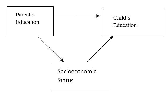
Regarding the relationship between the parent’s education level and respondent’s education level, the literature usually posits a positive relationship: That is, studies have found that parents with higher education levels, on average, have children with higher education levels (Kean-Davis, 2005). Kean Davis (2005) further finds that the reason for the correlation likely is a function of the belief and expectations that parents have for the children: this relationship, however, is, once again, mediated by the variable of socioeconomic status.

Diagram 2: Relationship between Parent’s and Child’s education mediated by Socioeconomic Status

Although this general positive relationship holds in many circumstances, there are notable exceptions.  For example, children of immigrants typically achieve a higher level of education than their parents.  Indeed, Hao and Bonstead-Bruns (1998) found that Asian immigrant children had higher levels of academic achievement and educational achievement than their parents; however, this effect was not observed seen across all immigrant groups (Hao & Bonstead-Bruns, 1998).  Thus, while one would generally expect to see a positive correlation between parent and child education, it would also heavily depend on the population being examined.  Detangling the causality between an individual parent’s involvement in education and the impact on a child’s is more difficult. Indeed, most studies show that a father’s educational level is positively linked to a child’s educational level; however, the direction of causality is not clear.  For example, more educated fathers tend to be more involved in their child’s education (once again mediated by socioeconomic status); at the same time, involvement is a key variable in predicting educational achievement and level in children (McBride, 2006). In general, a father’s education level and involvement is considered more important vis-à-vis his children.

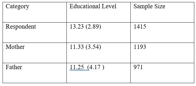
A descriptive analysis of the data set revealed that mothers (M= 11.33, SD=3.54) had a slightly higher level of education than the fathers (M=11.25, SD=4.17) of the respondents (M=13.23, SD=2.89). There is also a slight but noticeable difference in the samples size between the three variables- I decided to use pairwise exclusion as the guiding principle for analyzing the data.  That is, the literature suggests that the education level of the respondent is tied to the educational levels of both the father and mother.  Thus, first two dependent t-tests will be performed to see if there is a statistically different relationship between the respondent’s education level and the education of level of the father and mother, respectively. The null hypothesis in both dependent t-tests is the mean education level between the respondent and respective parent is equal.  The alternate hypothesis in both dependent t-tests is that the mean education level between the respondent and respective parent is not equal.

Table 2: Descriptive Statistics for Mean Educational Levels

There is also the existing problem discussed earlier in the paper: That is, all three variables in this analysis are interval variables, and are not continuous in nature.  In addition, the data points are not likely independent of each other- that is, the respondent’s education level is not independent of his/her parent’s education level. Thus, in order to deal with these problems, we will implement a similar strategy as question 1: First, a two-sample dependent t-test will be performed to gain understanding of the potential relationship between the two variables. Second, a Wilcoxon Signed-ranks test will be performed.  The tests will establish if the respondent’s education level is significantly different from each parent; after that, additional tests will be performed in order to figure out which parent has greater explanatory power vis-à-vis the respondent’s education level.
The null hypothesis in both dependent t-tests is the mean education level between the respondent and respective parent (mother and father) is equal.  The alternate hypothesis in both dependent t-tests is that the mean education level between the respondent and respective parent is not equal. A dependent samples t-test indicate that scores for the respondent (M=13.23, SD=2.89) was significantly higher than that for the respondent’s mother (M=11.33, SD=3.54)., t(1189)= 22.42, p<.000. Another dependent samples t-test indicate that scores for the respondent (M=13.23, SD=2.89) was significantly higher than that for the respondent’s father (M=11.25 SD=4.17), t (974) =19.57, p<.000.   It should be noted there was a fairly substantial loss of power when conducting the independent t-test sample vis-à-vis the respondent’s father due to the sample size.    From these tests, one concludes that the respondent’s education level differs from both parents.

A Wilcoxon Signed-rank test indicated that the respondent’s education level was significantly different from the mother’s educational level, Z=-19.358, p<.000, r=.40. A Wilcoxon Signed-rank test indicated that the respondent’s education level was significantly different from the father’s educational level, Z= -16.885, p<.000, r=.375.

There is still a question, however, on which parent’s education level has more of an influence on the respondent’s educational level.  In order to explore this question, two scatter plots were analyzed with the independent variable (maeduc or paeduc) on the x-axis and the respondent’s education level on the y-axis.  For this data set, the mother’s educational level seems to play a bigger role than the father’s educational level in influencing the respondent’s education level: The father’s education level only explained roughly 14% of the variation in the respondent’s education, Pearson’s r (974) =.40  p<.001; the mother, on the other hand, explained roughly 16% of the variation in the respondent’s education, Pearson’s r (1194) = .375 p<.001.

Linear relationship between age and education

The relationship between age and education has evolved over time, particularly in the United States.  Indeed, the correlation between age and education has evolved with different policies in education. There was a slightly positive correlation when associate degrees were first introduced, and many older and working individuals acquired a higher education level (Smith, 1996). However, as college and post-graduate education became more common decades after, the correlation between the two variables became increasingly negative. That is, younger individuals, on average, had a higher education level than older individuals.   This is most likely due to the influence of cohort effects- educational attainment has increased across generations during the 20th century (Smith, 1993).  Indeed, recent analyses conducted from General Social Surveys and American Election studies show a Pearson’s correlation of -.250 to-.295 for the relationship between age and education (Smith, 1993).

This question explores the linear relationship between the age of individuals in the study and their education levels (measured in highest year completed). The mean age of individuals in the study was roughly 47 (mean=46.56; standard deviation= 17.30); the mean of the highest year of school completed (mean=13.23; standard deviation=2.90).  In the model run for linear regression, the independent variable is age; the dependent variable is education.

Table 3: Descriptive Statistics for Mean Educational Levels

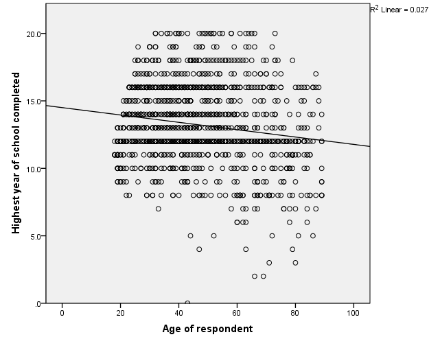
In order to obtain an approximate idea of the linear relationship between the two variables, a scatterplot was computed to assess the relationship between age and education.  Overall, the scatterplot showed a weak positive correlation between the variable, r=.17, n=1417, p=.000.  Overall, the scatterplot does not show a robust linear relationship.

Figure 1: Scatterplot of age on education

The next question is whether running a linear regression analysis is appropriate for these two variables. The variables need to meet the following assumptions for linear regression:   1) linearity of the relationship between dependent and independent variables; 2) independence of the errors; 3) homoscedasticity; 4) normality of the error distribution.  In order to check the linearity, a residual p-p plot and residual plot were graphed.

Figure 2: P-P Plot

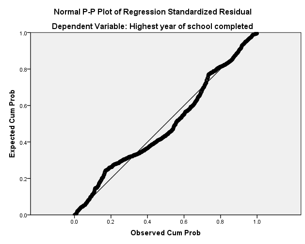
Figure 3: Residuals

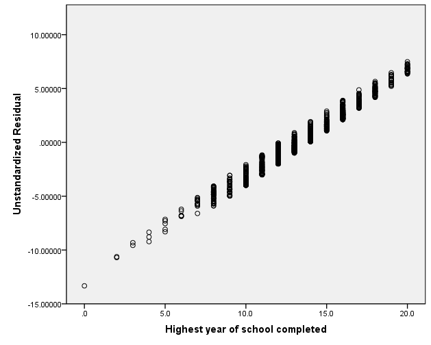
While these graphs do not show a clear linear relationship,  there is roughly linear relationship illustrated in the two graphs.  Regarding the remaining assumptions, the residuals show a borderline case (likely due to an interval variable), so the regression will be done, however, there will be a number of caveats to the final results. In this linear regression, the null hypothesis is that age is a predictor of education; the alternate hypothesi is that age is not a predictor of education.

A linear regression was used to test the hypothesis that age is a predictor of education.  The overall model proved significant in that R= -.163 F(1 ,1411)= 37.68, P<.000. As age increased, there was a decrease in educational level (B=14.502, SEB =.218, ? = -.027, p<.001). Overall, this equation extrapolates that an extra year in age would lead to a -.027 decrease in an individual’s age level.   There are two caveats to this linear regression model: 1) Age only explains roughly 2.6% of the variance in education; this is quite low.  2)  The use of the linear model is probably not appropriate for individuals that are very young or very old; that is, for individuals not necessarily in the data set.  Thus, age has a negative relationship to education level.

Relationship between marital status and education

The relationship between marital status and education is difficult to generalize due to potential mediators and confounders   For example, married men are usually better educated and have a higher income than single men (Sweeney, 2002).  However, the relationship between income and education is different for single women.

Diagram 3: Relationship between marital status and education- Men

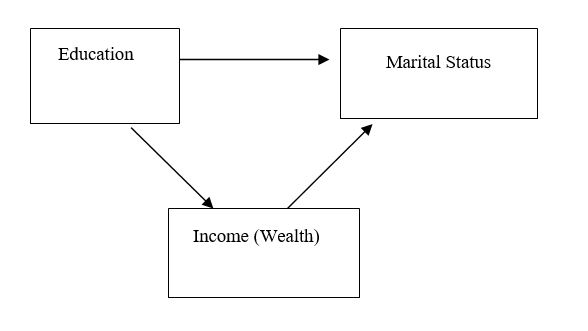
In contrast, single women tend to be better educated, and have higher income than married women (Sweeney, 2002). However this relationship is also moderated by a number of factors including time spent in the labor force and race (Sweeney, 2002).

Diagram 4: Relationship between marital status and education- Women

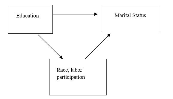
Thus, as in other relationships related to this data set, it is quite difficult to compare two variables without interaction for other factors such as labor participation and race, data we do not have access to. That correlation, however, is decreasing as the numbers of women increasingly have college education, as well as the need for stable income in order for a marriage to last (Musick, Brand & Davis, 2011).
In this example, the dependent variable is marital status and the independent variable is education. The dependent variable is categorical: that is, there are six categories, but they are not categorized in a natural fashion. As explored earlier in the paper, education years of the respondent is an interval variable; there is also another variable (highest degree received) that will allow us to check this relationship.  Thus, this relationship can be best explored through using the chi-squared test.

There are two issues, however, before actually conducting the test.  The assumptions needed in order to conduct a chi-squared test are two-fold: 1) The sample size must exceed 5 (n>5); 2) The sample must be randomly selected from the population.  The first assumption is clearly true in this data set; and there is an assumption that the second is likely true.  The null hypothesis for the chi-squared test is the relationship between being educational level and marital status is independent (no relationship between the two variables). The alternate hypothesis is there is a relationship between educational level and marital status.

There are two different ways to conduct a chi-squared test in this data set: 1) Use the integral variable educ (highest years of education-interval); 2) use the variable degrees earned (categorical). The first chi-squared test using years of education as the dependent variable  resulted in the respondents marital status did differ by educational status, l ?2(76, N =1415) =164.41, p<.001. However, due to the large number of degrees of freedom, I also ran the second test using finished degrees as a proxy for education, ?2(16, N =1411=64.01, p<.001.  Both tests suggest the null hypothesis should be rejected and the alternate hypothesis should be accepted: that is, there is a relationship between marriage status and educational level.

In order to determine whether married or singles have a higher education level in the data set, an independent samples t-test was conducted on married and single individuals in the sample. An independent samples t-test indicated that education levels for married individuals (M=13.48, SE=2.81) were higher than woman (M=13.64; SE=2.73), t (988)=-.88. p=.379.  Thus, we fail to reject the null hypothesis that educational levels for married and single individuals are equal, and conclude that married individuals have a higher education level in the data set.

References

McBride, B.A. (2005).  The Mediating Role of Fathers’ School Involvement on Student Achievement. Applied Development Psychology. 26(2): 201-216.

Kean-Davis, P.E. (2005). The influence of parent education and family income on child achievement: The indirect role of parental expectations and the home environment.  Journal of Family Psychology. 19(2), 294-304.

Hao, L. & Bonstead-Bruns, M. (1998). Parent-Child Differences in Educational Expectations and the Academic Achievement of Immigrant and Native Students. Sociology of Education, 71(3), 175-198.

Jacobs, J (1996).  Gender inequality and higher education. Annual Review in Sociology.  22, 153-185.

Mammen, K. & Paxson, C. (2000).  Women’s Work and Economic Develpoment.  The Journal of Economic Perspectives.  14(4), 141-164.

Musick, K., Brand, J.E. & Davis, D. (2011).  Variation in the relationship between education and marriage: mismatch in the marriage market.

Smith, T.W. (1993).  The relationship of age and top education across time.  Social Science Research.  22, 300-311.

Smith, T.W. (1997).  Examining the relationship between educational attainment, age/cohort, and dependent variables.  University of Chicago Methodological Report, 90.

Sweeney, M.M. 2002. “Two Decades of Family Change: The Shifting Economic Foundations of Marriage.” American Sociological Review, 67(1):132-147.