The Capital Asset Pricing Model, Research Paper Example

Summary

Capital Asset Pricing Model (CAPM) attempts to explain how to estimate the risk of cash flow from a possible investment project and assess the cost of capital on the project. According to this theory, these differences come from the differences in the risk of the returns on the assets.

Data for the study was secondary data collected from 109 out of over 2000 companies listed on New York Stock Exchange. Data was analyzed using descriptive statistics such as mean and standard deviation and the results presented using pie charts and graphs.

Results showed that there may be some existed multicollinearity problems between money supply and GDP and between GDP and income using correlation. On the other hand, using variance inflation factor showed that multicollinearity exists in the independent variable of money supply and income. In addition, although the VIF value of GDP is high, it doesn’t exceed 10, thus no multicollinearity problem for GDP.

Introduction

Background of the study

Capital Asset Pricing Model is used to determine a theoretically appropriate required rate of return of an asset. It takes into account the asset’s sensitivity to non-diversifiable risk which is the systematic or the market risk which is represented by beta in financial industry, as well as expected return of the market and expected return of a theoretical risk free asset.

This paper examines the validity of CAPM on the American stock market using monthly stock returns from 109 out of 2000 companies listed in the New York Stock Exchange from 31^st December 2008 to 31^st December 2011. New York Stock Exchange is by far the largest stock exchange by market capitalization of the listed companies in the whole world.

Research problem

The Capital Asset Pricing Model (CAPM) was introduced by Sharpe (1964) and Lintner (1965). It was a successful attempt to explain how to estimate the risk of cash flow from a possible investment project and assess the cost of capital on the project. According to this theory, these differences come from the differences in the risk of the returns on the assets. The theory claims that the accurate measure against riskiness is known as beta and the market risk premium per unit of riskiness is totally the same in all assets.

Objective

The main objective of the study is to examine the validity of the Capital Asset Pricing Model on the American stock market by use of monthly stock returns.

Research question

How valid is the Capital Asset Pricing Model on the American stock market using monthly stock returns?

Research hypothesis

H₀: The Capital Asset Pricing Model is valid on the American stock market using monthly stock returns

H₁: The Capital Asset Pricing Model is not valid on the American stock market using monthly stock returns

Methodology

This explains the procedure of carrying out the study. It includes; target population, sampling design, data collection procedures, data analysis and regression analysis.

Population of the study

The population targeted was companies listed in the New York Stock Exchange (NYSE) for the period dated 31^st December 2008 to 31^st December 2011.

Sampling design

109 companies out of over 2000 companies listed in the New York Stock Exchange were selected. Random sampling will be employed to avoid bias.

Data collection procedures

The study mainly relied on secondary data. This data was from New York Stock Exchange monthly stock returns for the period 31^st December 2008 to 31^st December 2011.Tests were conducted for 3 years (36 months) period using monthly stock returns.

Data analysis

The collected data was thoroughly examined and checked for completeness and comprehensibility. The data was then summarized and analyzed to generate descriptive statistics such as means, standard deviation and frequency distribution which will be used to analyze the data.

Regression model

Monthly stock returns were be given by;

rit= logPit-logPi (t-1)

where, rit= logarithmic return of stock I between time t-1 and t

Pit= closing price of stock i; on the first day of month t

Pi,t-1= closing price of stock i; on the first day of month t-1

The original Capital Asset Pricing Model is given by;

E (ri)-rf=?im (E (rm)-rf)

Where, E (ri) = expected return on stock

Rf= risk free rate of return

?im= systematic risk of stock

E (rm) = expected return on market portifolio

The next, Fama-MacBeth Approach:

Step 1 (First-Pass Regression):

For each of the N securities included in the sample, we first run the following regression over time to estimate beta:

Step 2 (Second-Pass Regression)

We run the following cross-section regression over the sample period over the N securities:

2.1  should not be significantly different from zero, or residual risk does not affect return.

2.2   should not be significantly different from zero, or the expected return on any asset is a positive linear function of its beta.

2.3    must be more than zero: there is a positive price of risk in the capital markets, namely, a positive relationship exists between systematic risk and expected return.

Discussion

The study was motivated by the need to examine the validity of the Capital Asset Pricing Model on American stock market using the monthly stock returns. The objective of the study was achieved by conducting a survey of 109 out of over 2000 companies listed in the New York Stock Exchange. Secondary data from the records of monthly stock returns was used.

Based on the previous researches, we are going to classify our variables into three categories: the macroeconomic factor includes GDP and CPI; the monetary factor is consisting of money supply and mortgage interest rate; the labor force factor has two components which are average income and unemployment rate. We then decide to use these predictors to establish a regression with Canadian housing price and figure out whether do these variables significantly affect the depend variable.

The regression model was performed on six variables, which are GDP, CPI, Mortgage Interest Rate, money supply, average income and unemployment rate. The SAS output is the following table.

GDP: Gross Domestic Product of Canada

CPI: Canadian Consumer Price Index

Interest: The mortgage interest rate of Canada

MS: The money supply M1 provided by Bank of Canada

Income: Canada total employees average hourly wages both sexes over 15 years

Unemp: The unemployment rate of the labor force in Canada

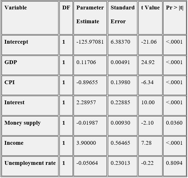
Figure 1

‘Best’ subset regression

In all-possible-regressions selection procedure, we select R-square, Adjusted R-square, Cp, AIC and SBC as the criteria. Based on the concept of the criteria, we choose the highest R-square, the lowest Cp value (or close to the number of p) and the lowest AIC and SBC.

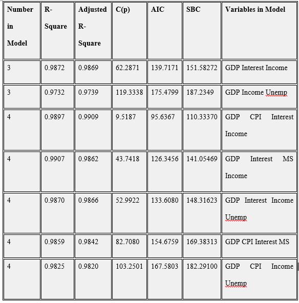
Figure 2

According to the SAS outputs above, the model with 5 variables which are GDP, CPI, Interest, MS, and income tend to be the optimal subset.

 Stepwise Regression

In the stepwise regression, we set the criterion for adding and deleting predictor variables as 0.01 and 0.15 respectively.

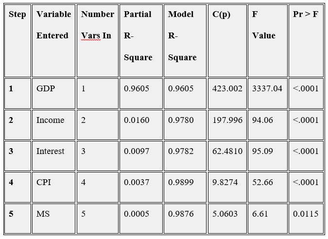
Figure 3

The results show that the subset consisting of GDP, income, interest, CPI and MS are selected, which conform to the results of the all-possible regression above.

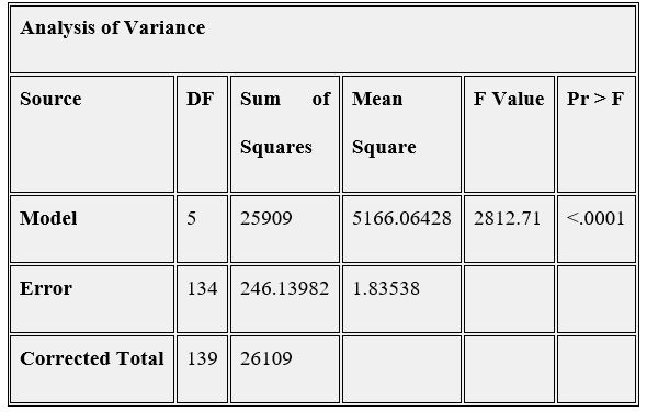
Figure 4

Second time stepwise

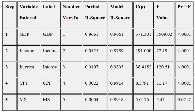
Figure 5

Correlation matrix

The correlation matrix shows the correlation for each two-variable combination, and this matrix can provide a general and overall view of the correlation between each variable. The output for the correlation matrix is shown below:

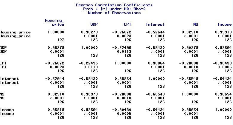
Figure 6

From the above table, with the correlation coefficient 0.98645, it is obvious that money supply is highly correlated with income. Besides, the correlation coefficients between money supply and GDP and between income and GDP are relatively high, 0.90379 and 0.93564 respectively, which indicate that there may be some existed multicollinearity problems between money supply and GDP and between GDP and income. The correlation matrix just provides the general view of the multicollinearity problem. It cannot give us the precise statistic analysis for this problem

Variance inflation factor

The VIF can measure the strength of the relationship between each explanatory variable in the regression. The largest VIF value among X variables is usually used to indicate the severity of multicollinearity and any individual VIF larger than 10 indicates that multicollinearity may be influential for least-squares estimates of the regression coefficients.

Figure 7

It is observed from the above table that the VIF values of money supply and income are 46.55611 and 67.04883, respectively, which indicates that multicollinearity exists in the independent variable of money supply and income. In addition, although the VIF value of GDP is high, it doesn’t exceed 10, thus no multicollinearity problem for GDP. Therefore, the variable of money supply was dropped from the model to fix the multicollinearity problem as money supply has less predicted power than income. Then the model is updated as follows:

New model

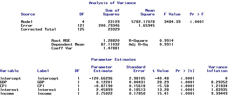
Figure 8

The study concludes that the error variance of the model is constant and the error terms also follow the normal distribution. The final regression model suggests that the housing price is affected by macroeconomic factors including GDP and CPI, monetary factor (mortgage interest rate) and labor force factor (income). Because of the largest t value, GDP displays the greatest influence on the housing price.

References

Lintner, J. (1965). The valuation of risk assets and the selection of risky investments in stock portfolios and capital budgets, Review of Economics and Statistics, 47 (1), 13-37.

Mullins, D.W. (1982). Does the capital asset pricing model work?, Harvard Business Review, January–February 1982, 105-113

Sharpe, William F. (1964). Capital asset prices: A theory of market equilibrium under conditions of risk, Journal of Finance, 19 (3), 425-442

Treynor, J.L. (1962). Toward a Theory of Market Value of Risky Assets. Unpublished manuscript. A final version was published in 1999, in Asset Pricing and Portfolio Performance: Models, Strategy and Performance Metrics. Robert A. Korajczyk (editor) London: Risk Books, pp. 15–22.